CNN Implementation Comparison

TensorFlow vs PyTorch for MNIST Classification

TensorFlow

PyTorch

This page compares two different implementations of a Convolutional Neural Network (CNN) for the MNIST digit classification task using pure TensorFlow and PyTorch. Both implementations achieve high accuracy while showcasing the unique features of each framework.

CNN Implementations

A detailed comparison of CNN implementations using TensorFlow and PyTorch for MNIST digit classification.

TensorFlow Implementation

Key Features

Pure TensorFlow

Implementation using low-level TensorFlow operations without Keras, providing full control over the architecture

Architecture

2 Convolutional layers (32 and 64 filters) with max pooling, followed by 2 fully connected layers

Training

Custom training loop with gradient tape for automatic differentiation

cnn_pure_tensorflow.py

Pure TensorFlow


                        // Code will be loaded via JavaScript

Implementation Analysis

Data Preprocessing

Normalizes pixel values to [0, 1] range
Reshapes data to include channel dimension
Converts labels to one-hot encoding
Handles batching for efficient training

Model Architecture

2 Convolutional layers (32 and 64 filters)
Max pooling for spatial dimension reduction
2 Fully connected layers (128 neurons, 10 output)
ReLU activation functions

Training Process

Custom gradient computation with GradientTape
Adam optimizer with 0.001 learning rate
Batch size of 128 for stable training
10 epochs of training

PyTorch Implementation

Key Features

Object-Oriented Design

Clean, modular implementation using PyTorch's nn.Module for better code organization

Dynamic Computation

Dynamic computational graphs for flexible model definition and easier debugging

Built-in Tools

Leverages PyTorch's DataLoader, optimizers, and loss functions

pytorch_cnn.py

PyTorch

Implementation Analysis

Data Management

Uses torchvision.datasets for MNIST loading
Custom normalization (μ=0.1307, σ=0.3081)
Parallel data loading with num_workers=2
Efficient batch processing with DataLoader

Network Structure

Identical architecture to TensorFlow version
Added dropout (0.25) for regularization
Dynamic input size calculation
Cleaner forward pass definition

Training Configuration

Smaller batch size (64) for better generalization
Same learning rate (0.001)
Explicit train/eval mode switching
Progress tracking with tqdm

Training Results

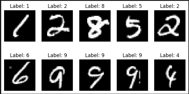
MNIST Dataset Visualization - Sample training images showing digit variety

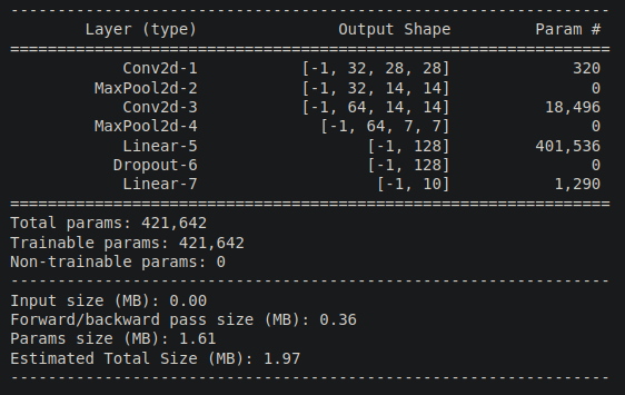
Model Architecture Summary - Layer-by-layer network structure

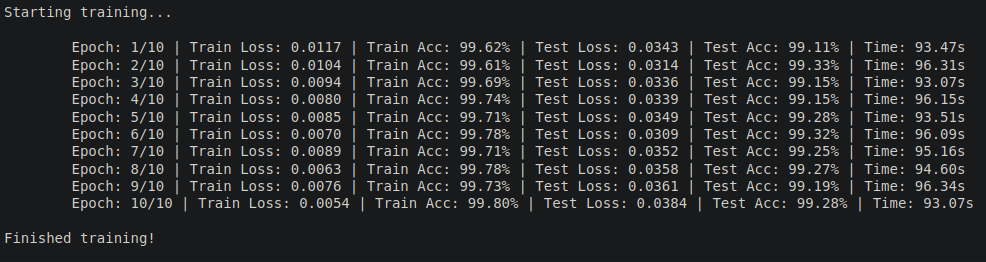
Training Progress - Epoch-wise training metrics

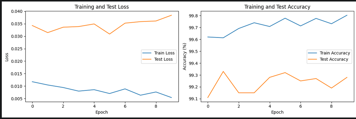
Loss and Accuracy Curves - Training convergence visualization

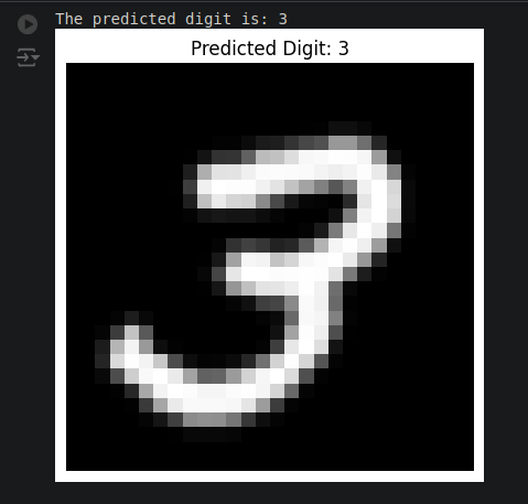
Model Predictions - Test set prediction examples

Framework Comparison

TensorFlow Advantages

Fine-grained control over operations
Explicit gradient computation
Efficient static graphs
Production-ready serving
Extensive visualization with TensorBoard

PyTorch Advantages

Intuitive object-oriented design
Dynamic computational graphs
Native Python integration
Easier debugging
More pythonic coding style

Code Comparison

TensorFlow Model


# TensorFlow CNN Model Definition
class CNNModel(tf.keras.Model):
    def __init__(self):
        super(CNNModel, self).__init__()
        # First Convolutional Block
        self.conv1 = tf.keras.layers.Conv2D(32, 3, activation='relu')
        self.pool1 = tf.keras.layers.MaxPool2D((2, 2))
        self.dropout1 = tf.keras.layers.Dropout(0.25)
        
        # Second Convolutional Block
        self.conv2 = tf.keras.layers.Conv2D(64, 3, activation='relu')
        self.pool2 = tf.keras.layers.MaxPool2D((2, 2))
        self.dropout2 = tf.keras.layers.Dropout(0.25)
        
        # Dense Layers
        self.flatten = tf.keras.layers.Flatten()
        self.dense1 = tf.keras.layers.Dense(128, activation='relu')
        self.dropout3 = tf.keras.layers.Dropout(0.5)
        self.dense2 = tf.keras.layers.Dense(10, activation='softmax')
    
    def call(self, x, training=False):
        # First Block
        x = self.conv1(x)
        x = self.pool1(x)
        if training:
            x = self.dropout1(x)
        
        # Second Block
        x = self.conv2(x)
        x = self.pool2(x)
        if training:
            x = self.dropout2(x)
        
        # Dense Layers
        x = self.flatten(x)
        x = self.dense1(x)
        if training:
            x = self.dropout3(x)
        return self.dense2(x)

PyTorch Model


# PyTorch CNN Model Definition
class CNNModel(nn.Module):
    def __init__(self):
        super(CNNModel, self).__init__()
        # First Convolutional Block
        self.conv1 = nn.Sequential(
            nn.Conv2d(1, 32, kernel_size=3),
            nn.ReLU(),
            nn.MaxPool2d(kernel_size=2),
            nn.Dropout(p=0.25)
        )
        
        # Second Convolutional Block
        self.conv2 = nn.Sequential(
            nn.Conv2d(32, 64, kernel_size=3),
            nn.ReLU(),
            nn.MaxPool2d(kernel_size=2),
            nn.Dropout(p=0.25)
        )
        
        # Dense Layers
        self.fc = nn.Sequential(
            nn.Flatten(),
            nn.Linear(64 * 5 * 5, 128),
            nn.ReLU(),
            nn.Dropout(p=0.5),
            nn.Linear(128, 10),
            nn.Softmax(dim=1)
        )
    
    def forward(self, x):
        x = self.conv1(x)
        x = self.conv2(x)
        return self.fc(x)

TensorFlow Data Loading


# TensorFlow Data Loading and Preprocessing
def load_and_preprocess_data():
    # Load MNIST dataset
    (x_train, y_train), (x_test, y_test) = tf.keras.datasets.mnist.load_data()
    
    # Normalize and reshape data
    x_train = x_train.astype('float32') / 255.0
    x_test = x_test.astype('float32') / 255.0
    
    # Add channel dimension
    x_train = x_train[..., tf.newaxis]
    x_test = x_test[..., tf.newaxis]
    
    # Create data pipeline
    train_ds = tf.data.Dataset.from_tensor_slices(
        (x_train, y_train)
    ).shuffle(10000).batch(32).prefetch(tf.data.AUTOTUNE)
    
    test_ds = tf.data.Dataset.from_tensor_slices(
        (x_test, y_test)
    ).batch(32).prefetch(tf.data.AUTOTUNE)
    
    return train_ds, test_ds

# Data Augmentation
data_augmentation = tf.keras.Sequential([
    tf.keras.layers.RandomRotation(0.1),
    tf.keras.layers.RandomZoom(0.1),
])

# Usage Example
train_ds, test_ds = load_and_preprocess_data()
for images, labels in train_ds:
    # Apply augmentation during training
    augmented_images = data_augmentation(images, training=True)
    # Train step...

PyTorch Data Loading


# PyTorch Data Loading and Preprocessing
def load_and_preprocess_data():
    # Define transformations
    transform = transforms.Compose([
        transforms.ToTensor(),
        transforms.Normalize((0.1307,), (0.3081,))
    ])
    
    # Data augmentation for training
    train_transform = transforms.Compose([
        transforms.RandomRotation(10),
        transforms.RandomAffine(0, translate=(0.1, 0.1)),
        transforms.ToTensor(),
        transforms.Normalize((0.1307,), (0.3081,))
    ])
    
    # Load MNIST dataset
    train_dataset = datasets.MNIST(
        './data', 
        train=True,
        download=True,
        transform=train_transform
    )
    
    test_dataset = datasets.MNIST(
        './data', 
        train=False,
        transform=transform
    )
    
    # Create data loaders
    train_loader = DataLoader(
        train_dataset,
        batch_size=32,
        shuffle=True,
        num_workers=2,
        pin_memory=True
    )
    
    test_loader = DataLoader(
        test_dataset,
        batch_size=32,
        shuffle=False,
        num_workers=2,
        pin_memory=True
    )
    
    return train_loader, test_loader

# Usage Example
train_loader, test_loader = load_and_preprocess_data()
for batch_idx, (data, target) in enumerate(train_loader):
    # Move to GPU if available
    data, target = data.to(device), target.to(device)
    # Train step...

TensorFlow Training


```python
# TensorFlow Training Loop
with tf.GradientTape() as tape:
    predictions = model(images, training=True)
    loss = loss_object(labels, predictions)
gradients = tape.gradient(loss, model.trainable_variables)
optimizer.apply_gradients(zip(gradients, 
                            model.trainable_variables))
```

PyTorch Training


```python
# PyTorch Training Loop
optimizer.zero_grad()
outputs = model(images)
loss = criterion(outputs, labels)
loss.backward()
optimizer.step()
```

Performance Analysis

Training Speed

Comparison of training time per epoch

Memory Usage

GPU memory consumption during training

Learning Resources

TensorFlow Resources

PyTorch Resources

Hamdi Abdeljawed

H.Abdeljawed

№ 2024

"Bridging the gap between TensorFlow and PyTorch, one implementation at a time."